* Creating Excel Container
Creating the Excel container, version 4.6.6.6.
The Excel container is now being selected. To do so, Data Container is clicked, then Excel. A name is chosen.

The name selected is "Dimension, Products." A description is added. Under Actions, all the actions that can be performed with the Excel spreadsheet are displayed.
In this case, the Read option is kept selected, and in the Name Path, the driver is chosen.

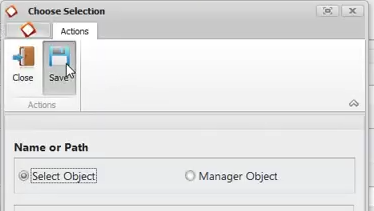
Clicking on Object, then Save, the driver is selected, and Save is clicked.


In Appointment File, the name of the Excel spreadsheet is entered. In the source directory, the Excel spreadsheet containing the product names is named Products.xlsx. Therefore, under Appointment Files, Products.xlsx is entered. Clicking New saves the data entered into the Excel Container component up to this point.

Next, Type Mapping is accessed. Here, the method for reading the spreadsheet is selected. There are four available options.
The chosen option is Direct Access Using Table Format. This means reading an Excel spreadsheet in table format. This format consists of the first row containing the name of each column, and from the second row onwards, the data is present.
Additionally, the Use Native Connection with Excel option is selected. This means a native PIS connection to Excel is used. This allows for reading without requiring Excel to be installed on the machine.

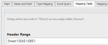
Since the Direct Access Using Table Format option was chosen, the configuration is done on the Mapping Table tab. Two parameters need to be specified: the range of cells for the spreadsheet header and the range of cells for the header data.
To specify these ranges, a range in Excel format is entered. This is an area of cells as Excel records these areas. To select these ranges, the spreadsheet is opened, and by dragging the mouse, the areas are selected.
Clicking the Preview button, the spreadsheet is displayed. This is why it's necessary to have Excel installed for these selections. Although Excel is not required for the reading itself.

The header ranges from cell A1 to cell P1. Therefore, this area is selected with a mouse drag.
With the spreadsheet open, the Range Cells button is clicked. This places the area into the configuration.

The sheet1 name is assigned to the spreadsheet, and it is copied from cell A1 to cell B1. The same process is repeated for the data range.

The data ranges from row 2 to row 36. However, to ensure a dynamic reading, only the first data row, row 2, is selected. Then the Get Data at First Empty Row option is chosen.

This option ensures that PIS will read all rows below row 2 within the column range (columns A and B) until it finds the first empty row.
After closing the Excel spreadsheet, the Update button is clicked with the selected range. A preview can be accessed by going to Excel Preview Table.

After clicking Preview, the list of products is displayed. Clicking Update again completes the successful reading of the spreadsheet with the list of products.


The next steps involve transformations to break down the descriptor into three new pieces of data: brand, flavor, and size. Following this, the lookup is applied under the brand descriptor.